Handle channel indices

Probes can have a complex contacts indexing system due to the probe layout. When they are plugged into a recording device like an Open Ephys with an Intan headstage, the channel order can be mixed again. So the physical contact channel index is rarely the channel index on the device.

This is why the Probe object can handle separate device_channel_indices.

Import

import numpy as np
import matplotlib.pyplot as plt

from probeinterface import Probe, ProbeGroup
from probeinterface.plotting import plot_probe, plot_probe_group
from probeinterface import generate_multi_columns_probe

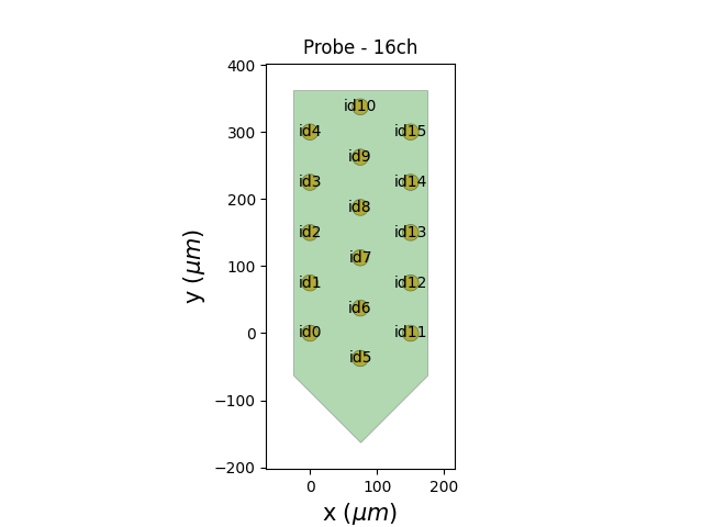
Let’s first generate a probe. By default, the wiring is not complicated: each column increments the contact index from the bottom to the top of the probe:

probe = generate_multi_columns_probe(num_columns=3,
                                     num_contact_per_column=[5, 6, 5],
                                     xpitch=75, ypitch=75, y_shift_per_column=[0, -37.5, 0],
                                     contact_shapes='circle', contact_shape_params={'radius': 12})

plot_probe(probe, with_contact_id=True)

(<matplotlib.collections.PolyCollection object at 0x7f6b983272b0>, <matplotlib.collections.PolyCollection object at 0x7f6b98218130>)

The Probe is not connected to any device yet:

print(probe.device_channel_indices)

None

Let’s imagine we have a headstage with the following wiring: the first half of the channels have natural indices, but the order of the other half is reversed:

channel_indices = np.arange(16)
channel_indices[8:16] = channel_indices[8:16][::-1]
probe.set_device_channel_indices(channel_indices)
print(probe.device_channel_indices)

[ 0  1  2  3  4  5  6  7 15 14 13 12 11 10  9  8]

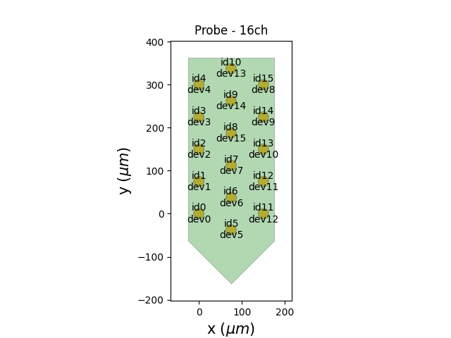
We can visualize the two sets of indices:

• the prbXX is the contact index ordered from 0 to N

• the devXX is the channel index on the device (with the second half reversed)

plot_probe(probe, with_contact_id=True, with_device_index=True)

(<matplotlib.collections.PolyCollection object at 0x7f6b9a54a5f0>, <matplotlib.collections.PolyCollection object at 0x7f6b98236e00>)

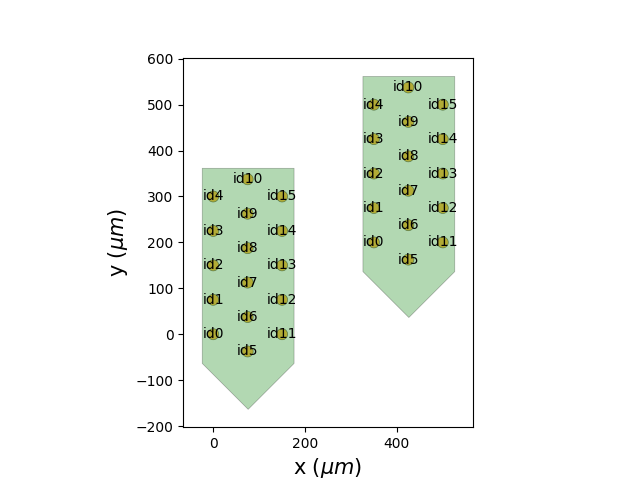
Very often we have several probes on the device and this can lead to even more complex channel indices. ProbeGroup.get_global_device_channel_indices() gives an overview of the device wiring.

probe0 = generate_multi_columns_probe(num_columns=3,
                                      num_contact_per_column=[5, 6, 5],
                                      xpitch=75, ypitch=75, y_shift_per_column=[0, -37.5, 0],
                                      contact_shapes='circle', contact_shape_params={'radius': 12})
probe1 = probe0.copy()

probe1.move([350, 200])
probegroup = ProbeGroup()
probegroup.add_probe(probe0)
probegroup.add_probe(probe1)

# wire probe0 0 to 31 and shuffle
channel_indices0 = np.arange(16)
np.random.shuffle(channel_indices0)
probe0.set_device_channel_indices(channel_indices0)

# wire probe0 32 to 63 and shuffle
channel_indices1 = np.arange(16, 32)
np.random.shuffle(channel_indices1)
probe1.set_device_channel_indices(channel_indices1)

print(probegroup.get_global_device_channel_indices())

[(0, 12) (0, 15) (0,  8) (0, 14) (0,  6) (0, 10) (0,  1) (0,  3) (0,  4)
 (0,  5) (0, 13) (0,  0) (0,  2) (0,  7) (0,  9) (0, 11) (1, 28) (1, 16)
 (1, 22) (1, 30) (1, 26) (1, 27) (1, 18) (1, 25) (1, 24) (1, 31) (1, 17)
 (1, 20) (1, 23) (1, 29) (1, 19) (1, 21)]

The indices of the probe group can also be plotted:

fig, ax = plt.subplots()
plot_probe_group(probegroup, with_contact_id=True, same_axes=True, ax=ax)

plt.show()