Plot values

Here is an example of how to plot values with color scales. And also to plot an interpolated image.

from pprint import pprint

import numpy as np
import matplotlib.pyplot as plt

from probeinterface import Probe, get_probe
from probeinterface.plotting import plot_probe

Download one probe:

manufacturer = 'neuronexus'
probe_name = 'A1x32-Poly3-10mm-50-177'

probe = get_probe(manufacturer, probe_name)
probe.rotate(23)

fake values

values = np.random.randn(32)

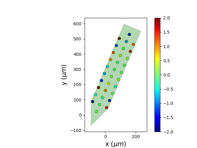
plot with values

fig, ax = plt.subplots()
poly, poly_contour = plot_probe(probe, contacts_values=values,
            cmap='jet', ax=ax, contacts_kargs={'alpha' : 1},  title=False)
poly.set_clim(-2, 2)
fig.colorbar(poly)

<matplotlib.colorbar.Colorbar object at 0x7f4781079bd0>

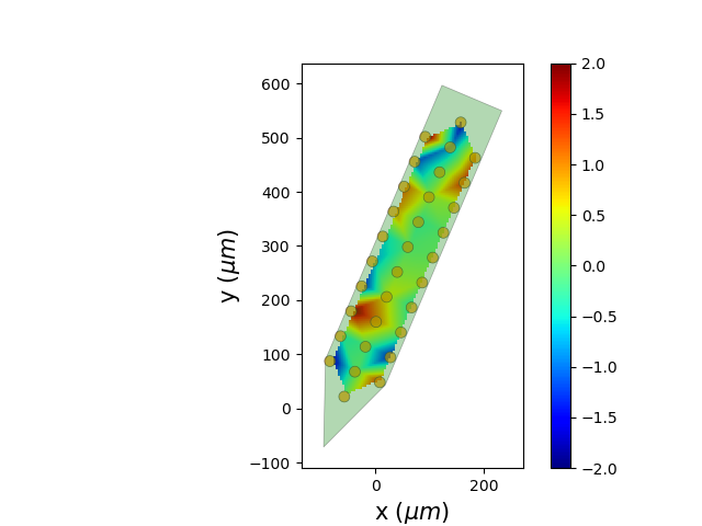
generated an interpolated image and plot it on top

image, xlims, ylims = probe.to_image(values, pixel_size=4, method='linear')

print(image.shape)

fig, ax = plt.subplots()
plot_probe(probe, ax=ax, title=False)
im = ax.imshow(image, extent=xlims+ylims, origin='lower', cmap='jet')
im.set_clim(-2,2)
fig.colorbar(im)

(127, 67)

<matplotlib.colorbar.Colorbar object at 0x7f477ae18820>

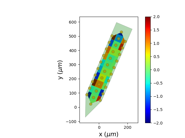
works with several interpolation methods

image, xlims, ylims = probe.to_image(values, num_pixel=1000, method='nearest')

fig, ax = plt.subplots()
plot_probe(probe, ax=ax, title=False)
im = ax.imshow(image, extent=xlims+ylims, origin='lower', cmap='jet')
im.set_clim(-2,2)
fig.colorbar(im)



plt.show()